
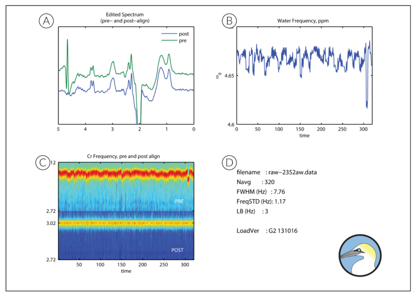
A. The plot top left shows the processed GABA-edited difference spectrum, the key output of the GannetLoad module. This plot shows the spectrum before frequency and phase correction above in green and the spectrum after frequency and phase correction below in blue. Hopefully the spectrum below should look nicer than the spectrum above.
B. The plot top right shows the frequency of the maximum point in the spectrum (usually residual water signal) plotted against time. Time is measured at the resolution of time-resolved data is fed in. The y-axis is free to scale according to the data, so be sure to check the y-range. This information can be interpreted in several ways, but it gives qualitative information on the stability of the experiment, e.g. field drift, subject motion, accuracy of prospective frequency correction etc. Field drift will appear as a non-zero slope in this trace, and movement as a discontinuity in the trace. Some datapoints may be circled in red in this plot. These are datapoints that have been rejected – see more below.
C. The plot bottom left presents the Cr signal over the duration of the experiment (same x-axis as B). The y-axis here represents the frequency in ppm of the Cr signal. The spectra at each timepoint are presented as a vertical stripe in the image, color-coded according to signal intensity, so the Cr signal should appear as a ‘hot’ stripe running through the image. In the upper half (PRE), the stripe should vary in frequency in a similar fashion to the water plot in B. In the lower half (POST), the result of frequency and phase correction (default is spectral registration SR3) is shown and ideally a more uniform horizontal stripe should appear. In the lower half (POST), some rows will appear as a dark blue stripe (i.e. no Cr peak at all). These rows, corresponding to the red circled points in B, have been rejected because one of the fitting parameters used for frequency correction lie more than three standard deviations from the mean. When an outlier is identified for rejection, rejection is always performed pairwise, i.e. if an OFF scan is rejected, a neighbouring ON scan will also be rejected, so as to balance the number of OFFs and ONs for subtraction.